Image Pyramids and Background Subtraction
Gaussian and Laplacian pyramids from scratch, single vs multi-frame background subtraction, and connected components.
Abstract#
Two topics in this one. The first half is building Gaussian and Laplacian image pyramids from scratch, which was mostly about getting the resize function to work correctly with scikit-image’s affine transforms. The second half is background subtraction: first with a single reference frame, then with a statistical model built from 30 frames, followed by morphological cleanup and connected component labeling.
Gaussian pyramid#
A Gaussian pyramid is a stack of progressively smaller, blurrier copies of an image. You smooth the image, downsample it by half, smooth again, downsample again. Each layer is half the resolution of the one above it.
The smoothing kernel comes from class. You compute where:
I reused the 1D Gaussian filter from HW2. With you get int(4 * 0.5 + 0.5) = 2, so the kernel has entries: [0.05, 0.25, 0.4, 0.25, 0.05]. That matches the kernel from the slides. The smooth function applies this with scipy.ndimage.gaussian_filter, which does the 1D convolution along each axis separately.
from scipy import ndimage as ndi

def smooth(image, sigma):
    smoothed = np.empty(image.shape, dtype=np.double)
    ndi.gaussian_filter(image, sigma, output=smoothed)
return smoothedThe resize function was more work. For downscaling you just take every other pixel. For upscaling (which the Laplacian pyramid needs later), you double the image size but fill the new rows and columns with zeros. I used skimage.transform.AffineTransform for this:
from skimage.transform._geometric import AffineTransform
from skimage.transform._warps import warp

def resize(image, output_shape):
    # ... estimate affine transform from 3 control points ...

    # fill alternating rows/cols with 0 instead of interpolating
    tform.params[0, 1] = 0
    tform.params[1, 0] = 0

    out = warp(image, tform, output_shape=output_shape)
return outSetting tform.params[0, 1] = 0 and tform.params[1, 0] = 0 is the part that matters. Without those lines, the affine warp interpolates between pixels when it upscales. With them, a (2, 2) image stretched to (4, 4) looks like:
             | a | 0 | b | 0 |
             ----------------
             | 0 | 0 | 0 | 0 |
 |a|b|       ----------------
 -----  -->  | a | 0 | b | 0 |
 |a|b|       ----------------
| 0 | 0 | 0 | 0 |You want the zeros because the smoothing step fills them in. If you let the warp interpolate, you’re smoothing twice.
Both gaussian_pyramid and laplacian_pyramid are generators. Each call to next() gives you the next layer down. I wrote them with yield so you don’t have to allocate all layers up front.
def pyramid_down(image, downscale=2):
    image = img_as_float(image)
    out_shape = tuple([math.ceil(d / float(downscale)) for d in image.shape])
    smoothed = smooth(image, sigma=0.5)
    out = resize(smoothed, out_shape)
    return out

def gaussian_pyramid(image, max_layer=-1, downscale=2):
    image = img_as_float(image)
    prev_layer_image = image
    yield image

    layer = 0
    current_shape = image.shape
    while layer != max_layer:
        layer += 1
        layer_image = pyramid_down(prev_layer_image, downscale)

        prev_shape = np.asarray(current_shape)
        prev_layer_image = layer_image
        current_shape = np.asarray(layer_image.shape)

        if np.all(current_shape == prev_shape):
            break

yield layer_imagemittens = imread('./data/murder_mittens.png')
gray_mitts = rgb2gray(mittens)
pyramid = tuple(gaussian_pyramid(gray_mitts, max_layer=3))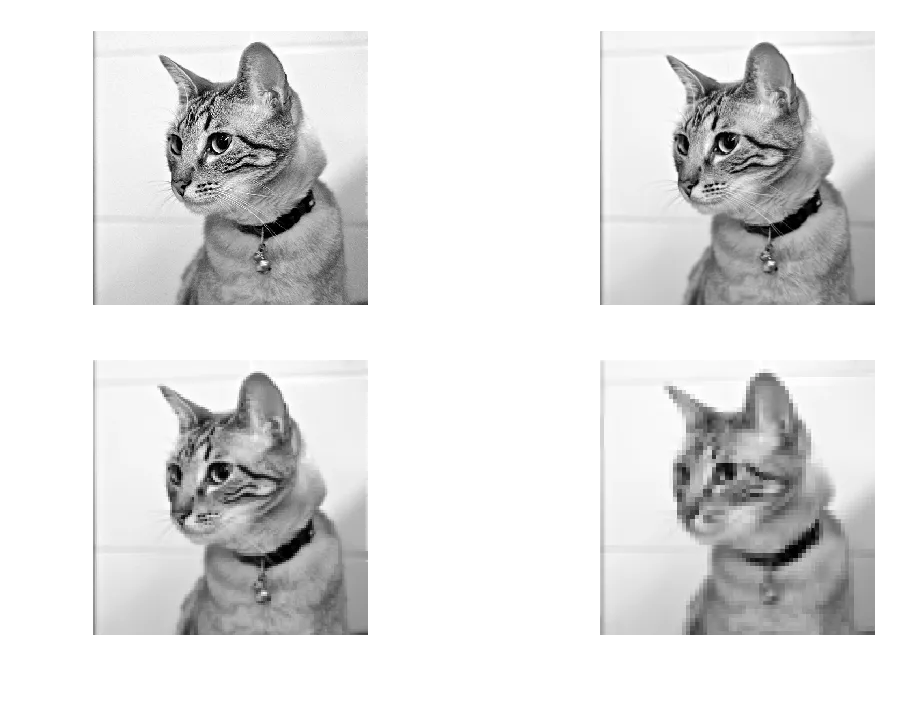
Gaussian pyramid, 4 layers. Each layer is half the resolution of the previous one.
Laplacian pyramid#
The Laplacian pyramid stores the difference between each layer and a smoothed version of itself. Each layer is: original at that scale minus the smoothed version. So it captures what the smoothing removed. Edges, textures, that kind of thing.
def laplacian_pyramid(image, max_layer=-1, downscale=2):
    image = img_as_float(image)
    sigma = 0.5
    current_shape = image.shape
    smoothed_image = smooth(image, sigma)

    yield image - smoothed_image

    if max_layer == -1:
        max_layer = int(np.ceil(math.log(np.max(current_shape), downscale)))

    for layer in range(max_layer):
        out_shape = tuple(
            [math.ceil(d / float(downscale)) for d in current_shape])
        resized_image = resize(smoothed_image, out_shape)
        smoothed_image = smooth(resized_image, sigma)
        current_shape = np.asarray(resized_image.shape)

        yield resized_image - smoothed_image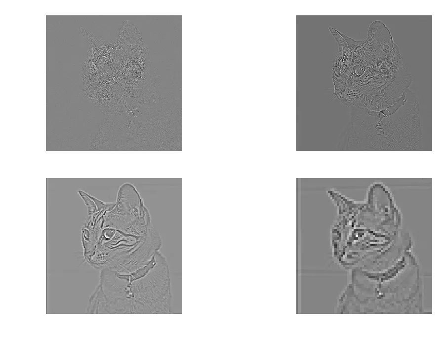
Laplacian pyramid, 4 layers. The first layer has the most detail (edges of the cat’s fur). Later layers are mostly flat.
The first layer is mostly edges. You can see the outline of the cat, whiskers, the pattern on the fur. By layer 3 and 4 there’s almost nothing left because there’s not much fine detail at that resolution.
The Gaussian and Laplacian pyramids are inverses of each other. You can reconstruct the original image by adding the Laplacian layers back up through the Gaussian pyramid. I didn’t implement reconstruction here since it wasn’t part of the assignment.
Background subtraction: single frame#
Now the background subtraction part. The data is a set of 30 frames of an empty scene (bg000.bmp through bg029.bmp) and one frame with a woman walking through it (walk.bmp).
Start simple: take one background frame and the test frame, compute the absolute difference per pixel, threshold it.
background = img_as_float(imread('./data/bg000.bmp'))
woman = img_as_float(imread('./data/walk.bmp'))

diff = np.abs(np.subtract(woman, background))

threshLevels = [0.15, 0.25, 0.3, 0.50, 0.65, 0.75]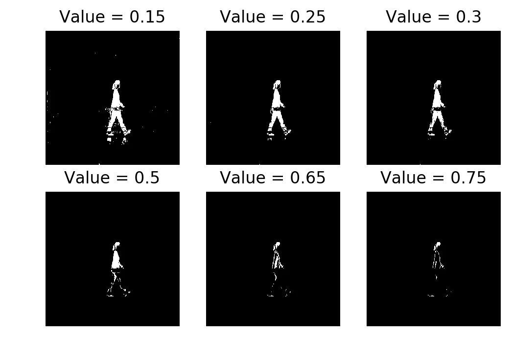
Single-frame subtraction thresholded at 0.15, 0.25, 0.3, 0.50, 0.65, 0.75
Thresholds 0.25 and 0.3 do a reasonable job. You can see the person. At 0.15 there are specks of activation everywhere because even small lighting variations between the two frames pass the threshold. At 0.75 you only get a few fragments of the person’s clothing where the color difference from the background is large.
If you tried to do morphological cleanup on the 0.15 result, the noise would probably merge into blobs that aren’t the person. On 0.75 the person would disappear entirely. You need the threshold to be in a narrow range, and with one reference frame you’re just guessing.
Background subtraction: multiple frames#
Now use all 30 background frames. Stack them into a cube, compute the per-pixel mean and standard deviation across frames.
background_cube = []
for i in range(30):
    tmp = img_as_float(imread('./data/bg{:03}.bmp'.format(i)))
    background_cube.append(tmp)

background_cube = np.array(background_cube)
background_mean = np.mean(background_cube, axis=0)
background_std = np.std(background_cube, axis=0) + 0.1The + 0.1 on the standard deviation is to avoid division by zero. Some pixels have identical values across all 30 frames (like a patch of wall that never changes), so their std is 0.
Now instead of a simple difference, you compute a Mahalanobis-like distance:
A pixel that’s 2 standard deviations from the mean background is suspicious. A pixel that’s 5 standard deviations away is almost certainly foreground.
diff_mahalanobis = np.divide(
    np.square(np.subtract(woman, background_mean)),
    np.square(background_std))

threshLevels = [2, 4, 8, 16, 24, 32]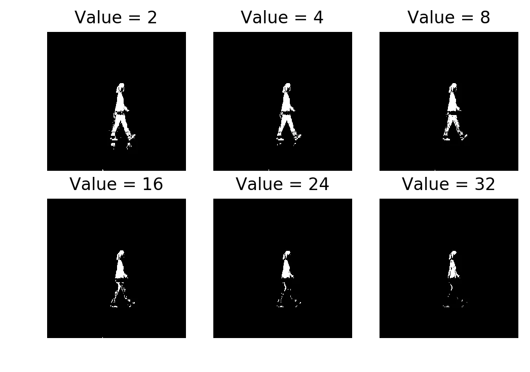
Multi-frame subtraction (Mahalanobis distance) thresholded at 2, 4, 8, 16, 24, 32
The difference from single-frame is obvious. Even at (more than ) the upper body of the person is still detected. You’d never use a significance level that extreme in normal statistical analysis. But the per-pixel standard deviation is so tight on static background regions that even a moderate intensity change is many away.
Single-frame subtraction compares against one reference frame. If that frame had slightly different lighting, you’d over-detect or under-detect and there’s nothing you can tune. The multi-frame model averages out those frame-to-frame variations.
Morphological closing#
Take the thresholded result (at ) and apply morphological closing with a square structuring element.
from skimage.morphology import closing, square

plt.imshow(closing(thresh, square(3)), cmap='gray')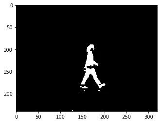
After closing: gaps filled, person is a mostly-solid blob
Closing is dilation followed by erosion. Dilation expands white regions, filling in small holes. Erosion shrinks them back so the overall size stays about the same. The result is that small gaps inside the person get filled in.
The hip region is still broken. That’s a quirk of the image (the person’s clothing matches the background color there), not of the model.
Connected components#
Last step: label the connected regions and overlay them on the original image.
from skimage.segmentation import clear_border
from skimage.measure import label
from skimage.color import label2rgb
from skimage.morphology import dilation

bw = dilation(thresh, square(3))
cleared = clear_border(bw)
label_image = label(cleared)
image_label_overlay = label2rgb(label_image, image=woman)

plt.imshow(image_label_overlay)clear_border removes any components touching the image edge (those are usually not the object of interest). label assigns an integer to each connected region. label2rgb colors each region and overlays it on the original.
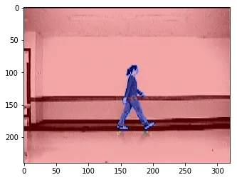
Connected components overlaid on the original frame. The person is one component (blue).
The person shows up as a single connected component. You could pull a bounding box from regionprops at this point, but the assignment didn’t ask for that.
What I got out of this#
The pyramids were mostly about getting the resize function right. The math is simple (smooth, downsample, repeat) but the implementation with AffineTransform was finicky. I had to read the skimage source to figure out the tform.params trick for zero-filling.
The background subtraction part was more interesting. The jump from single-frame to multi-frame is just “use statistics instead of a single reference,” but the difference in output is large. The single-frame method needs you to pick the right threshold and even then it’s fragile. The multi-frame method works across a wide range of thresholds because the per-pixel standard deviation captures how much each pixel normally varies.