
Fractals for Image Classification Feature Extraction
Exploring how fractal geometry, specifically Hilbert curves, can provide a novel approach to feature extraction in image classification.
Introduction: Rethinking Feature Extraction with Fractals#
Feature extraction is at the core of image classification, a task that has seen groundbreaking advancements thanks to convolutional neural networks (CNNs). These models have revolutionized computer vision by leveraging spatial coherence to extract patterns, enabling machines to distinguish cats from dogs, recognize handwritten digits, and even detect tumors in medical scans. However, as powerful as CNNs are, they come with limitations—particularly their reliance on convolution operations, which are heavily tuned for two-dimensional data.
What if there were an alternative to convolutions? One that could preserve spatial relationships while offering a fresh perspective on how we process and interpret image data? Enter fractals, the infinitely complex, self-replicating structures that bridge mathematics and nature. In this blog post, I’ll explore how fractal geometry, specifically the Hilbert curve, can provide a novel approach to feature extraction.
This method reimagines image processing by transforming pixel data into a dense, one-dimensional representation using fractal-based mappings. Unlike traditional techniques, it takes advantage of the Hilbert curve’s ability to preserve locality and scale across resolutions, making it ideal for compact, efficient feature representation. Combined with wavelet transforms, which localize features in the frequency domain, this fractal-based approach opens up exciting possibilities for image classification and beyond.
Fractals: A brief overview#
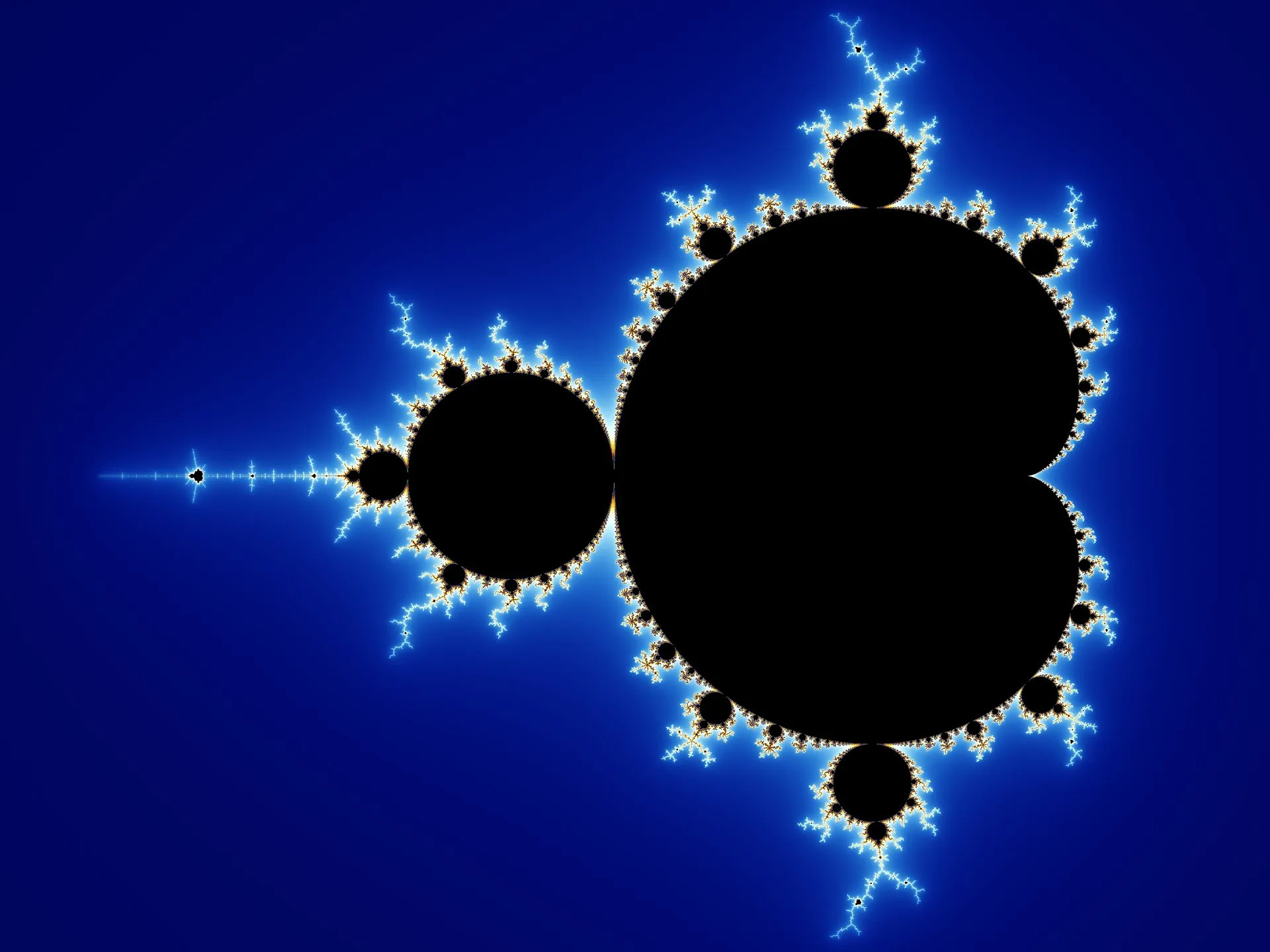
A fractal is an abstract object used to describe and simulate naturally occurring objects. The proper definition of a fractal, at least as Mandelbrot wrote it, is a shape whose “Hausdorff dimension” is greater than its “topological dimension”. Topological dimension is something that’s always an integer, wherein (loosely speaking) curve-ish things are 1-dimensional, surface-ish things are two-dimensional, etc. For example, a Koch Curve has topological dimension 1, and Hausdorff dimension 1.262. A rough surfaces might have topological dimension 2, but fractal dimension 2.3. And if a curve with topological dimension 1 has a Hausdorff dimension that happens to be exactly 2, or 3, or 4, etc., it would be considered a fractal, even though it’s fractal dimension is an integer.
For purposes of my method we can simplify our view of fractal as essentially a never-ending pattern. But even under fractals, there is a special set of self-similar fractals. These are rendered by repeating a simple process. The interesting property about fractals is that they exist in non-whole number dimensions, as discussed above (The Hausdorff dimension). This property is super-useful as this means that they effectively encode information from a non-primary dimension, a fact that was used extensively for lossy image compression.
We can use to our advantage this property to capture spatial, temporal or higher dimensional relation- ships in form of useful features that can be localized. (Using something like a Fourier transform or as in our case, wavelet transform)
Space-Filling Curves and Practical Applications#
Before diving into the technicalities, let’s talk about space-filling curves. These are mathematical constructions that, despite their counterintuitive nature, are immensely useful. A space-filling curve is a line that weaves through every point in a two-dimensional (or higher-dimensional) space. One famous example is the Hilbert curve, which can be visualized as a fractal that becomes progressively more intricate at higher resolutions.
Bridging Infinite and Finite Realities#
Space-filling curves address a philosophical question central to mathematics: How can results based on infinite concepts be useful in our finite world? The Hilbert curve provides a fascinating answer. It starts as a theoretical construct, existing in an infinite, continuous mathematical space. But its finite approximations—pseudo-Hilbert curves—serve practical purposes, such as translating images into sound or encoding spatial information into dense, one-dimensional representations.
Let me illustrate with an example: Imagine developing a device that helps people “see with their ears.” The device takes data from a camera, translates it into sound, and lets users interpret spatial information through auditory cues. In this setup, the Hilbert curve provides a way to map 2D image data (pixels) into a 1D frequency space, preserving spatial relationships between pixels while creating a coherent auditory representation.
Fractals in Feature Extraction: The Proposed Methodology#
Fractals, with their self-similar and infinitely intricate structures, provide a powerful framework for extracting meaningful features from complex datasets like images 1. The goal is to transform 2D image data into a dense, 1D representation that preserves spatial relationships and is optimized for computational efficiency. This section breaks down the methodology into three key components: mapping pixels to frequencies, employing the Hilbert curve for serialization, and leveraging wavelet transforms for localization and compression.
From Pixels to Frequencies: Bridging the Dimensions#
At the heart of the method is the challenge of mapping two-dimensional pixel data to a one-dimensional frequency domain. Each pixel is associated with a frequency, and its intensity determines the loudness of that frequency in the resulting signal. This transformation enables image data to be represented as a superposition of frequencies, much like a musical composition where different instruments (frequencies) contribute to the overall sound 2.
The challenge lies in ensuring that this mapping preserves spatial coherence. Pixels that are close together in the original image should remain close in the frequency representation 3. This is critical for maintaining the integrity of spatial relationships, which are often key to successful image classification. Without this coherence, the resulting representation would lose its ability to accurately capture the structure of the original image.
Comparing Space Filling Curves#
Space-filling curves provide a structured way to map multi-dimensional data into one-dimensional representations while attempting to preserve spatial locality. However, not all space-filling curves are created equal. When choosing a curve for applications like image feature extraction, it’s crucial to evaluate their performance in preserving spatial relationships. Let’s compare three popular curves: the Z-curve, the Peano curve, and the Hilbert curve. 4
The Z-Curve#
The Z-curve, or Morton order, follows a zig-zag pattern that makes it simple to implement but poor at preserving spatial relationships. In 2D, the Z-curve introduces significant gaps, with many adjacent points in the sequence mapping to coordinates that are far apart in the original space. This results in an average displacement for unit edges exceeding 1.6 in 2D and 1.35 in higher dimensions, making it unsuitable for applications requiring strong locality preservation.Peano Curve#
The Peano curve, in contrast, is much better at maintaining spatial coherence. By mapping scalar unit lengths in 1D to unit Euclidean lengths in 2D, it ensures that horizontal segments are exactly one unit long, although vertical segments can stretch to 2 or 5 units, slightly raising the average displacement. The Peano curve also achieves asymptotic stability at higher ranks, with its performance aligning closely with the Hilbert curve as resolution increases.Hilbert Curve#
Hilbert curve stands out as the best option for preserving locality. Its recursive, self-similar structure ensures that adjacent points in the sequence remain as close as possible in the original space, outperforming the Peano curve in both horizontal and vertical coherence. The Hilbert curve also scales well to higher dimensions, maintaining its locality-preserving properties regardless of resolution. Studies such as Color-Space Dimension Reduction and Bongki 2001 consistently rate the Hilbert curve as the superior choice, edging out the Peano curve in overall performance.Implementation#
To achieve a mapping that preserves spatial relationships, I turn to the Hilbert curve, a type of fractal known as a space-filling curve. The Hilbert curve provides an elegant solution to the problem of mapping 2D space to 1D space while preserving locality. Here’s why it’s so effective:
-
Locality Preservation: Points that are close together on the Hilbert curve are also close together in the 2D image. This ensures that nearby pixels are mapped to nearby frequencies, preserving spatial coherence.
-
Scalability: The Hilbert curve is recursive and self-similar, meaning it can scale to any resolution. Whether the image is 256x256 or 512x512 pixels, the curve adapts seamlessly, providing a consistent framework for feature extraction.
-
Stability Across Resolutions: As the resolution of an image increases, the points on the Hilbert curve move less and less. This stability is crucial for applications where the resolution may change over time, such as progressive updates to image datasets or hierarchical processing pipelines.
The Process of Hilbertification#
Hilbertification refers to the process of mapping an image's pixel data to a 1D representation using the Hilbert curve. Here's how it works:-
Divide the Image into Quadrants: The Hilbert curve starts by dividing the image into smaller regions, or quadrants, and defining a path that traverses each quadrant in a specific order.
-
Recursive Subdivision: Each quadrant is further subdivided into smaller grids, with the Hilbert curve path becoming increasingly intricate. This process repeats until the curve has visited every pixel in the image.
-
Generate a 1D Sequence: The final result is a 1D sequence of pixel intensities, where the order of the pixels reflects the traversal path of the Hilbert curve. This sequence forms the input for subsequent signal processing steps.
Wavelet Transforms for Feature Localization and Compression#
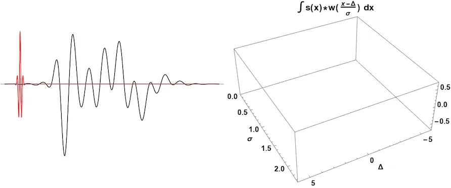
After Hilbertification, the next step is to apply wavelet transforms, which are mathematical tools for analyzing signals at multiple scales. Unlike Fourier transforms, which only provide frequency information, wavelet transforms capture both frequency and spatial (or temporal) information, making them ideal for feature extraction in images.
Experimentation#
Support vector machines (SVMs) are a set of supervised learning methods used for classification, regression and outliers detection. The advantages of support vector machines are that they are effective in high dimensional spaces, still effective in cases where number of dimensions is greater than the number of samples, use a subset of training points in the decision function (called support vectors), so it is also memory efficient and versatile due to them supporting different Kernel functions which can be specified for the decision function. 5 This was then followed by hilbertification, which is the process of serializing the image to the frequency domain as discussed earlier. This was then passed onto for localization. The fundamental idea of wavelet transforms is that the transformation should allow only changes in time extension, but not shape, this means that it encapsulates a denser representation of our signal on the time domain such that it preserves the spatial relationships as changes in the time extension are expected to conform to the corresponding analysis frequency of the basis function 6. This gives us a more dense set of features which is 1/4 the size of the original image.

Table below gives an overview of how my proposed method performs. Note that for my tests I had taken the entire image as a baseline. Apart from the documented results show below, I have also compared my method to cosine-transformed version of the dataset, in which case the result of the cosine-transformed classifiers were abnormally low so I decided to not publish those as it maybe due to my own faulty implementation I had also tried CIFAR-10 dataset, since that dataset is a color dataset, I did not get time to properly implement the method for the dataset.
Results of the Proposed Method#
| Dataset | Method | Linear SVM | RBF Kernel | Polynomial Kernel |
|---|---|---|---|---|
| Fashion MNIST | Hilbertified | 87.273 | 88.275 | 87.991 |
| Baseline | 91.493 | 89.917 | 91.584 | |
| MNIST | Hilbertified | 96.026 | 96.535 | 97.134 |
| Baseline | 98.318 | 98.661 | 99.288 |
Conclusions#
In order to reduce the number of features that are being considered while classification is done and still achieve a better accuracy levels, I applied hilbertification to the dataset and then used wavelets to localize the features thus giving us a denser set of features almost one-fourth of the original image. The results that I saw was not significantly lower when compared to the results obtained while considering all the features. Thus, it can be said that my method indeed captures the spatial relationships as proposed. Based on this, I have come to believe that the proposed method is not only viable, it also encodes some of very useful spatial information in a very dense space. This method can be extended extensively in future work by expanding to higher number of dimensions since it can efficiently encode temporal and spatial and even higher order dimensional data.
Footnotes#
-
Falconer, Kenneth (2003). “Fractal Geometry: Mathematical Foundations and Applications.” John Wiley & Sons. xxv ISBN 0-470-84862-6. ↩
-
von Melchner, Laurie & Pallas, Sarah & Sur, Mriganka (2000) “Visual Behaviour Mediated by Retinal Projections Directed to the Auditory Pathway.” Nature 404 871-6. 10.1038/35009102. ↩
-
Boeing, G. (2016). “Visual Analysis of Nonlinear Dynamical Systems: Chaos, Fractals, Self-Similarity and the Limits of Prediction.” Systems 4 (4): 37. doi:10.3390/systems4040037. ↩
-
Jaffer, Aubrey. “Color-Space Dimension Reduction.” Accessed November 19, 2018. https://people.csail.mit.edu/jaffer/CNS/PSFCDR ↗. ↩
-
Alex J. Smola, Bernhard Scholkopf. “A Tutorial on Support Vector Regression.” Statistics and Computing archive Volume 14 Issue 3, August 2004, p. 199-222. ↩
-
Chui, Charles K. (1992). “An Introduction to Wavelets.” San Diego: Academic Press ISBN 0-12-174584-8. ↩