
Soft-Margin SVMs: Linear and Kernel
Implementing soft-margin linear SVM and polynomial kernel SVM from scratch with gradient descent, grid search over learning rates and regularization.
Abstract#
Two SVMs from scratch on the same MNIST-like binary classification data. The linear SVM uses hinge loss with L2 regularization and hits 96% accuracy. The kernel SVM uses a degree-3 polynomial kernel in a dual formulation and gets 91%. The linear SVM won, which wasn’t what I expected. Grid search over learning rates and lambda values for both.
Same dataset as the logistic regression post: 784-dimensional binary MNIST data, about 6100 training samples, separate validation and test sets. This time two classifiers, both SVMs, both implemented with NumPy and no external ML libraries.
Soft-margin linear SVM#
The hinge loss#
The SVM uses hinge loss instead of logistic loss:
Plus an L2 regularization term added to the gradient (not to the risk computation, which only tracks the hinge loss itself).
The hinge loss is zero when , meaning the sample is on the correct side of the margin. The “soft margin” part is that we allow some samples to violate the margin, penalizing them linearly instead of requiring perfect separation.
Subgradient descent#
The hinge loss isn’t differentiable at , so technically this is subgradient descent. For each sample where the hinge condition is violated (), we accumulate into the gradient:
def calculate_gradient(w, lamda):
    gradient = np.zeros((1, 784), dtype=np.float128)
    for i in range(N):
        xi = trainingData[i]
        yi = trainingLabels[i]
        if yi * np.dot(w, xi.T) < 1:
            gradient += -yi * xi
    gradient = gradient / N
    gradient += lamda * w
return gradientClassification is just the sign of : positive means class , non-positive means class .
Grid search#
I searched over 54 combinations: 9 learning rates 6 lambda values, each run for iterations. Most of the larger learning rates produced garbage (50-90% error), but a few combinations in the low learning rate range worked well.
Best hyperparameters: learning rate = 5e-6, lambda = 0.001.
| Metric | Training | Validation | Test |
|---|---|---|---|
| Error | 3.26% | 3.96% | 3.88% |
| Accuracy | 96.74% | 96.04% | 96.12% |
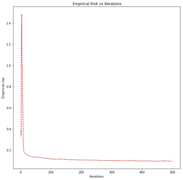
Hinge loss decreasing over 500 iterations for the best hyperparameters.
Validation and test accuracy are within 0.1% of each other. The model generalizes well, and the regularization is doing its job preventing overfitting on 784 features.
Compared to logistic regression (which achieved a test risk of 0.119 but didn’t report classification accuracy directly), the linear SVM at 96.1% accuracy is a strong baseline for a linear model. Both are finding linear boundaries in 784-dimensional space; the difference is in the loss function. The hinge loss focuses on samples near the decision boundary (the support vectors), while logistic loss penalizes all misclassified samples with a smooth curve.
Soft-margin kernel SVM#
The polynomial kernel#
The kernel SVM works in a higher-dimensional feature space without computing the transformation explicitly. I used a degree-3 polynomial kernel:
The division by 784 normalizes for the feature dimension. Without it, the dot products of 784-dimensional vectors are large, and raising them to the third power makes everything explode.
The data also needed normalization before computing kernels:
trainingData_norm = (trainingData / 128.0) - 1.0This maps pixel values from to . The logistic regression and linear SVM worked on raw pixel values, but the kernel SVM is more sensitive to scale because the polynomial kernel amplifies differences.
Dual formulation#
Instead of optimizing a weight vector directly, the kernel SVM optimizes dual coefficients (one per training sample) and a bias . The prediction for a new point is:
The gradient of involves the precomputed kernel matrix (an matrix of all pairwise kernel values between training samples). For each training point where the hinge condition is violated, we accumulate kernel-weighted gradients plus an L2 regularization term:
def calculate_gradient_a(a, k_a_b, lamda):
    gradient = np.zeros((N, 1), dtype=np.float128)
    for p in range(N):
        yp = trainingLabels[p]
        if 1 - yp * k_a_b[p] > 0:
            gradient += (-yp * k[p].T).reshape(N, 1)
    gradient = gradient / N
    gradient += (lamda / 2) * np.dot((k + k.T), a)
return gradientThe bias gradient is simpler: sum for all hinge-violated points, divide by .
Grid search#
120 combinations: 12 learning rates 10 lambda values, iterations each. This took a while. The kernel matrix alone is , and every gradient computation touches the full matrix.
Most combinations with learning rates below 1e-4 didn’t learn anything (stayed at ~46% error, the prior class distribution). The model only started learning with learning rates of 1e-3 and above.
Best hyperparameters: learning rate = 1, lambda = 1e-7.
| Metric | Training | Validation | Test |
|---|---|---|---|
| Error | 7.67% | 8.0% | 9.3% |
| Accuracy | 92.33% | 92.0% | 90.7% |
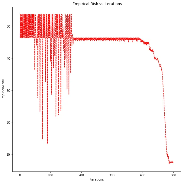
Classification error decreasing over 500 iterations for the best kernel SVM hyperparameters.
Comparing the three classifiers#
| Classifier | Test Error | Test Accuracy |
|---|---|---|
| Logistic Regression | (risk: 0.119) | — |
| Linear SVM | 3.88% | 96.12% |
| Kernel SVM | 9.30% | 90.70% |
The linear SVM outperformed the kernel SVM, which wasn’t what I expected going in. The kernel SVM maps the data into a higher-dimensional space (degree-3 polynomial features), which should give it more expressive power. But more expressive power also means more room to overfit, and the kernel SVM has far more parameters ( dual coefficients vs. 784 primal weights).
A few things probably contributed to the kernel SVM underperforming:
-
The grid search wasn’t as thorough. Most of the 120 combinations failed to learn anything. The good region of the hyperparameter space was narrow (learning rate near 1, lambda near 1e-7), and I might have missed better combinations.
-
500 iterations might not be enough. The kernel SVM’s loss was still decreasing at iteration 500. The linear SVM had mostly converged by then.
-
The data might be close to linearly separable. If the two digit classes can be separated by a hyperplane in 784 dimensions with only ~4% error, there isn’t much room for a nonlinear kernel to improve. The kernel adds complexity without enough payoff.
The linear SVM at 96% is hard to beat for the amount of effort. A simple hyperplane in pixel space, no feature engineering, no normalization needed. Sometimes the simple model wins.