
Logistic Regression Decision Boundaries
Building logistic regression from scratch in NumPy with gradient checking, feature scaling, and decision boundary visualization on exam data.
Abstract#
Implement logistic regression from scratch using only NumPy: sigmoid function, cost function, gradient checking, feature scaling, and batch gradient descent. Then use it to predict university admissions from two exam scores.
This assignment was about building logistic regression without any ML libraries. The dataset has 100 students with two exam scores each and a binary label for whether they got admitted. The goal is to learn a decision boundary that separates the two classes.
The data#
The dataset is simple: 100 rows, two features (Exam 1 score and Exam 2 score), and a binary label (admitted or not). Here’s what it looks like:
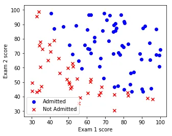
Exam 1 score vs Exam 2 score. Blue circles are admitted students, red x’s are rejected. There’s a rough diagonal separation between the two groups.
You can eyeball a boundary between the two clusters, but it’s not perfectly clean. A few blue dots sit in the red zone and vice versa.
Sigmoid function#
The sigmoid function maps any real number to the range , which makes it useful for modeling probabilities:
The implementation needs to handle numerical stability. If is very negative, explodes. If is very large and positive, we’re fine because goes to zero. The fix is to clip the input values to a safe range before computing:
def sigmoid(z):
    largest_float64 = 709.782712893384
    least_value_greater_zero = -36.04365338911715
    y = np.clip(z, -1 * largest_float64, -1 * least_value_greater_zero)
    s = 1 / (1 + np.exp(-1 * y))
return sThose magic numbers come from the limits of float64: 709.78 is and 36.04 is where is machine epsilon. Outside that range, the exponential either overflows or the result is indistinguishable from 0 or 1 anyway.
The gradient of sigmoid has a nice form. If , then:
def sigmoid_grad(f):
return f * (1 - f)This is one of those formulas that’s easy to derive but also easy to mess up in code if you forget that the input should be , not itself.
Cost function#
The logistic regression cost function (negative log-likelihood) for training examples is:
where is the hypothesis.
def cost_function(theta, X, y):
    z = np.dot(theta, X.T)
    h_x = sigmoid(z)
    cost = (-1.0 / len(y)) * np.sum(
        np.multiply(y, np.log(h_x)) +
        np.multiply(1 - y, np.log(1 - h_x))
    )
return costThe gradient with respect to works out to:
def gradient_update(theta, X, y):
    z = np.dot(theta, X.T)
    h_x = sigmoid(z)
    grad = np.zeros(theta.shape)
    for i in range(grad.shape[0]):
        term = np.multiply((h_x - y), X[:, i].T)
        grad[i] = np.sum(term)
    grad = grad / X.shape[0]
return gradGradient checking#
Before trusting the gradient computation, we verify it numerically using the centered difference approximation:
with . If the relative difference between the numerical and analytical gradients is less than , the gradient check passes.
def gradcheck_naive(f, x):
    rndstate = random.getstate()
    random.setstate(rndstate)
    fx, grad = f(x)
    h = 1e-4

    it = np.nditer(x, flags=['multi_index'], op_flags=['readwrite'])
    while not it.finished:
        ix = it.multi_index
        e = x.astype('float64')
        e[ix] += h
        random.setstate(rndstate)
        f_plus_epsilon, _ = f(e)
        e[ix] -= 2.0 * h
        random.setstate(rndstate)
        f_minus_epsilon, _ = f(e)
        numgrad = (f_plus_epsilon - f_minus_epsilon) / (2 * h)

        reldiff = abs(numgrad - grad[ix]) / max(1, abs(numgrad), abs(grad[ix]))
        if reldiff > 1e-5:
            print("Gradient check failed at index %s" % str(ix))
            return
        it.iternext()
print("Gradient check passed!")All six gradient checks passed (scalar, 1-D, and 2-D for a quadratic function, plus 1-D, 2-D, and range tests for sigmoid). The cost/gradient function also passed gradient checking on random data with 100 samples and 10 features.
Feature scaling and gradient descent#
Before running gradient descent, we need feature scaling. The exam scores range from roughly 30 to 100, and without scaling the gradient steps would be uneven across dimensions. The approach here is simple: divide each feature by its maximum absolute value, mapping everything to . We also prepend a bias column of ones (which stays at 1 after scaling by its own max).
The gradient descent update is the standard batch update:
The learning rate is set to and then multiplied by the number of training examples (100), making the effective rate 1.0. The algorithm runs for 400 iterations.
Here’s the decision boundary right at the start, when is random:
Iteration 1, cost = 0.703. The initial decision boundary is essentially random, cutting through the data without regard for the actual class separation.
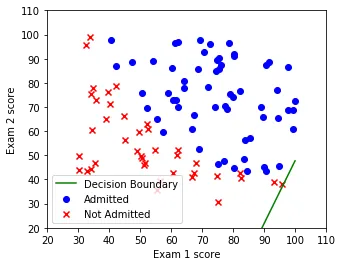
And after 400 iterations of gradient descent:

Iteration 400, cost = 0.329. The learned boundary separates the two classes reasonably well, running diagonally from upper-left to lower-right.
The cost decreased steadily from 0.703 to 0.329 over the 400 iterations. Here are some checkpoints:
| Iteration | Cost |
|---|---|
| 1 | 0.703 |
| 50 | 0.576 |
| 100 | 0.498 |
| 200 | 0.408 |
| 300 | 0.360 |
| 400 | 0.329 |
Prediction and accuracy#
The predict function applies the same feature scaling used during training, computes , and thresholds at 0.5:
def predict(theta, X):
    X_bias = np.ones((X.shape[0], X.shape[1] + 1))
    X_bias[:, 1:] = X
    X_bias = X_bias * 1.0 / train_max_values

    probabilities = sigmoid(np.dot(theta, X_bias.T))
    predicted_labels = (probabilities >= 0.5).astype(float)
return probabilities, predicted_labelsA few test cases:
- Exam scores (90, 90): probability 0.968, predicted admitted
- Exam scores (50, 60): probability 0.349, predicted not admitted
- Exam scores (50, 50): probability 0.237, predicted not admitted
The training accuracy comes out to 92.0%. That’s 92 out of 100 students classified correctly. For a linear model on a dataset that isn’t perfectly linearly separable, that’s a reasonable result.
What I learned#
The main takeaway from this assignment was how all the pieces of logistic regression fit together when you build them yourself. The sigmoid function, cost function, gradient computation, and gradient descent are all pretty short pieces of code on their own. The tricky parts are the numerical stability (clipping sigmoid inputs to avoid overflow) and remembering to apply the same feature scaling at prediction time as at training time. Gradient checking was also useful as a sanity check. It’s slow (you have to evaluate the cost function twice per parameter), but it catches sign errors and off-by-one mistakes that would otherwise be hard to track down.