Motion History Images and Optical Flow
Image differencing with morphological cleanup, MEI and MHI temporal representations, similitude moments on motion images, and Lucas-Kanade optical flow.
Abstract#
This assignment is about detecting and representing motion in video. It starts with frame differencing (absolute difference, threshold, morphological cleanup), then builds two temporal representations from the difference images: Motion Energy Images (cumulative OR) and Motion History Images (recency-weighted). I also computed similitude moments on both, reusing the function from HW4. The last part implements Lucas-Kanade optical flow on a synthetic test case.
Image differencing#
The idea is simple. Take two consecutive frames, subtract them, threshold the result. Pixels above the threshold are “motion.” The differencing function is:
I used the naive absolute difference instead of Weber’s difference. Tried six threshold values: 0.05, 0.08, 0.10, 0.12, 0.15, 0.2.
im1 = img_as_float(imread('./data/aerobic-001.bmp'))
im2 = img_as_float(imread('./data/aerobic-002.bmp'))

threshLevels = [0.05, 0.08, 0.10, 0.12, 0.15, 0.2]
f, axarr = plt.subplots(2, 3, sharex='col', sharey='row', dpi=200)
for thresh in threshLevels:
    magIm = np.abs(im1 - im2)
    tImg = magIm > thresh
    idx = threshLevels.index(thresh)
    axarr[int(idx/3), idx%3].axis('off')
    axarr[int(idx/3), idx%3].set_title(f'Value = {thresh}')
    axarr[int(idx/3), idx%3].imshow(tImg, cmap='gray', aspect='auto')
Raw frame differencing. The result is fractured at every threshold.
The raw difference image is noisy and broken up. Not usable for anything downstream. You need morphological operations to clean it up.
Morphological cleanup#
I tested four approaches on the difference image before thresholding. All used a square(5) structuring element.
Closing (dilation then erosion):
from skimage.morphology import closing, square

magIm = np.abs(im1 - im2)
magIm = closing(magIm, square(5))
tImg = magIm > thresh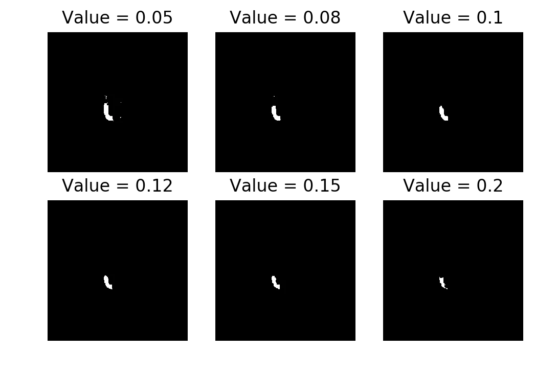
Closing. Fills in the gaps without expanding the region too much. Best result of the four.
Opening (erosion then dilation):

Opening. Fails because erosion runs first and destroys the fragmented regions.
Opening is almost entirely blank. The difference image is already fractured, so erosion first just wipes everything out. By the time dilation runs there’s nothing left to expand.
Dilation (alone):

Dilation only. Produces a visible silhouette but it’s chunky.
Dilation gives a reasonable shape but the regions are too fat. In a motion detection pipeline that would mean false positives around the edges.
Median filter:
from skimage.filters.rank import median

im1 = median(im1)
im2 = median(im2)
magIm = np.abs(im1 - im2)
tImg = magIm > thresh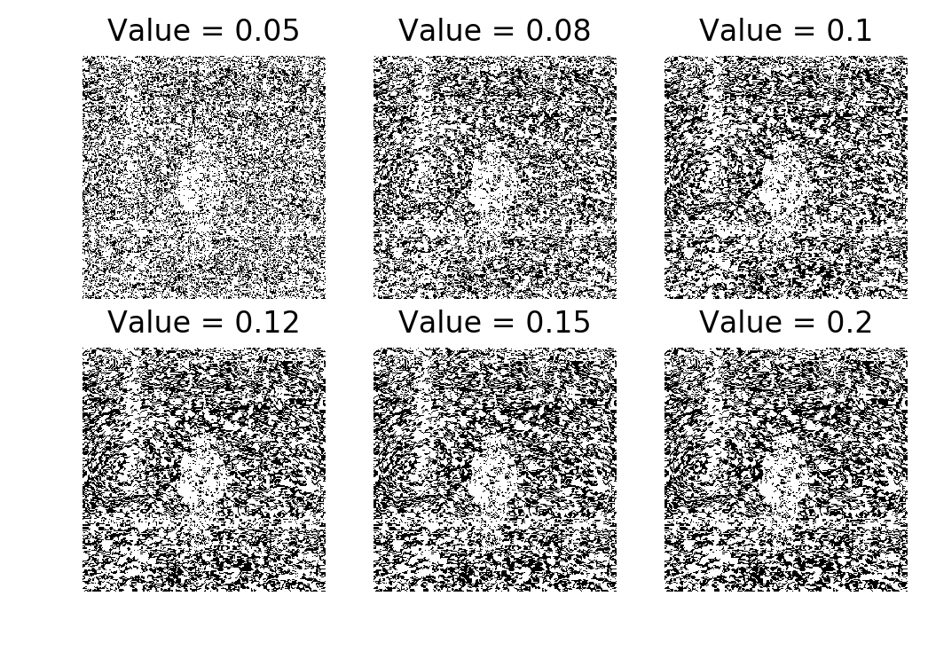
Median filter. Broken. There’s a precision loss warning (float64 to uint8) from skimage.
The median filter produced garbage. I got a UserWarning: Possible precision loss when converting from float64 to uint8 from skimage’s dtype conversion. I’m not sure if the implementation was wrong or if the float-to-uint8 conversion was killing it. Either way, the result was unusable.
Closing worked best. I used closing with threshold 0.08 for the rest of the assignment.
MEI and MHI#
Load all 22 frames and compute consecutive differences using closing + threshold 0.08:
aer_cube = []
for i in range(1, 23):
    tmp = imread('./data/aerobic-{:03}.bmp'.format(i))
    tmp = img_as_float(tmp)
    aer_cube.append(tmp)
aer_cube = np.array(aer_cube)

T = aer_cube.shape[0]

aer_diff = np.abs(aer_cube[1:,:,:] - aer_cube[:-1,:,:])
for i in range(aer_diff.shape[0]):
aer_diff[i] = closing(aer_diff[i], square(5)) > 0.08Here are all 21 consecutive differences laid out:
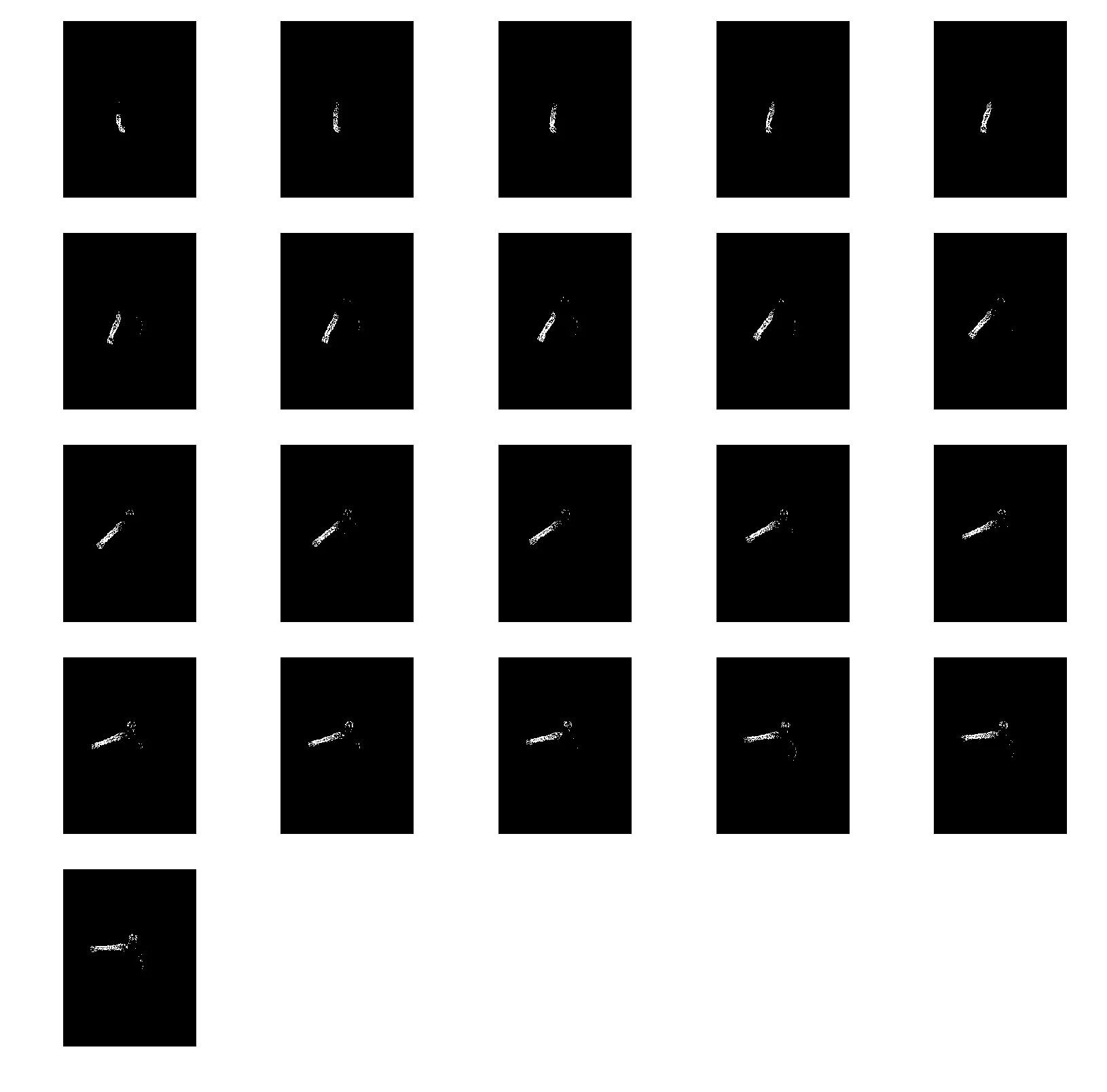
Consecutive frame differences (with closing + threshold 0.08). Each cell is . You can see the person’s limbs moving frame to frame.
These are the building blocks for both MEI and MHI below.
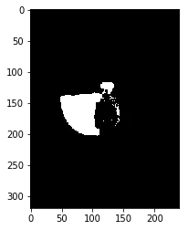
Motion Energy Image#
MEI is a cumulative OR of all difference frames up to time . If a pixel had motion at any point, it’s 1 in the MEI.
MEI = [aer_diff[:i, :, :].max(axis=0) for i in range(1, T)]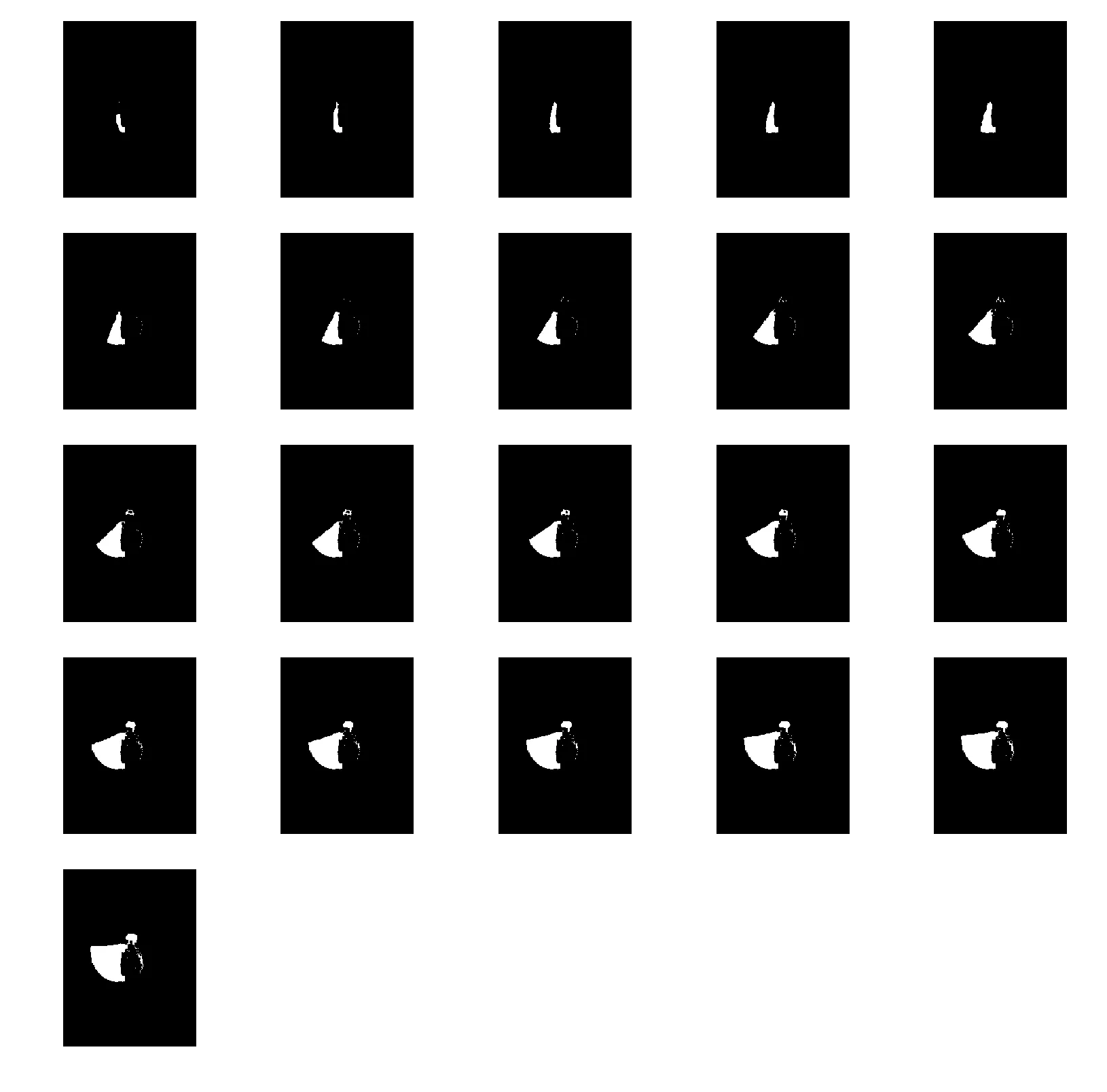
MEI accumulating over 21 frames. The silhouette grows as more motion is observed.
The MEI just keeps growing. By the last frame it’s a blob that covers everywhere the person moved. It tells you where motion happened but nothing about when.
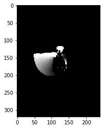
Motion History Image#
MHI assigns each pixel a recency value. If a pixel has motion at time , set it to (the max). Otherwise, decay it by 1 each frame (floored at 0).
MHI = np.zeros(aer_cube.shape)

for idx in range(1, T-1):
    for i in range(0, aer_cube.shape[1]):
        for j in range(0, aer_cube.shape[2]):
            if aer_diff[idx][i][j] == 1:
                MHI[idx][i][j] = T
            else:
MHI[idx][i][j] = max(0, MHI[idx-1][i][j] - 1)Yes, that’s a triple nested loop. In Python. It ran, but it was slow. The recurrence relation (MHI[idx] depends on MHI[idx-1]) makes it hard to vectorize cleanly, so I left it as-is.

MHI across 21 frames. Brighter pixels are more recent motion. The gradient encodes direction.
The MHI is more useful than the MEI. You can see the brightness gradient: recent motion is bright, older motion is darker. If the person’s hand is going up, the top of the trail is bright and the bottom is dim. If the hand is going down, it’s the opposite. The MEI would look the same either way.
I also computed the MHI with thresholding, where :
delta_T = (T - 15) / 8

MHI_deltaT = np.zeros(MHI.shape)
for idx in range(1, T-1):
    for i in range(0, aer_cube.shape[1]):
        for j in range(0, aer_cube.shape[2]):
            if MHI[idx][i][j] - delta_T > 0:
                MHI_deltaT[idx][i][j] = MHI[idx][i][j] - delta_T
MHI with . The subtraction removes old motion, keeping only the recent part of the trail.
Moments on MEI and MHI#
I reused the similitudeMoments() function from HW4 on the last frames of both representations. The MHI frame was normalized by , and the MEI was normalized by .
Final MHI frame (normalized by T).
Final MEI frame (normalized).
The MHI has a lower mean than the MEI because of the gradient. The MHI is smooth, with values fading from bright to dark, so the average pixel intensity is lower. The MEI is binary (a pixel is either 1 or 0), so within the motion region the values are all at the same level.
The other moment values between the two are similar. The shapes are similar since MHI is basically the MEI with a gradient painted on top.
Lucas-Kanade optical flow#
For the optical flow part, I tested on a synthetic example first. Two 101x101 black images, each with a 21x21 white box. The second box is shifted by 1 pixel down and 1 pixel to the right.
box1 = np.zeros((101, 101))
box2 = np.zeros((101, 101))

size = 21
box1[39:39+size, 5:5+size] = 1
box2[40:40+size, 6:6+size] = 1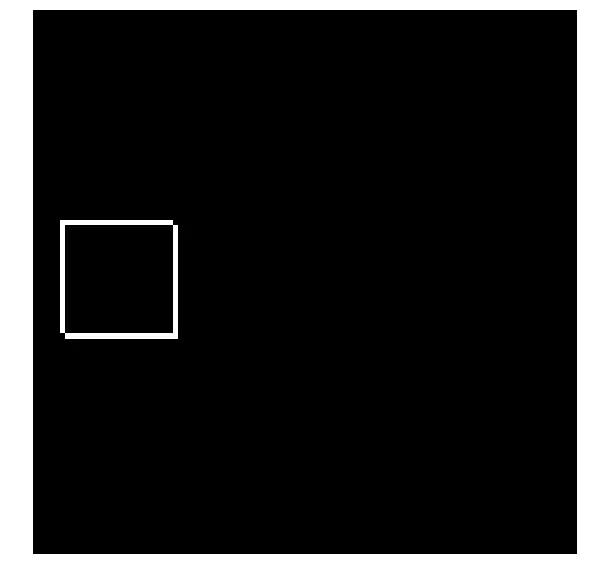
Absolute difference of the two box images. The L-shaped residual shows the 1-pixel shift.
The Lucas-Kanade method computes optical flow by solving the brightness constancy equation in a local window. You need the spatial gradients , and the temporal gradient . I computed these with 2x2 convolution kernels from the lecture slides:
from scipy import signal

def optical_flow(I1g, I2g, window_size):

    kernel_x = 0.25 * np.array([[-1., 1.], [-1., 1.]])
    kernel_y = 0.25 * np.array([[-1., -1.], [1., 1.]])
    kernel_t = 0.25 * np.array([[1., 1.], [1., 1.]])
    kernel_x = np.fliplr(kernel_x)
    mode = 'same'

    fx = signal.convolve2d(I1g, kernel_x, boundary='symm', mode=mode)
    fy = signal.convolve2d(I1g, kernel_y, boundary='symm', mode=mode)
    ft = (signal.convolve2d(I2g, kernel_t, boundary='symm', mode=mode) +
          signal.convolve2d(I1g, -kernel_t, boundary='symm', mode=mode))

    u = np.zeros(I1g.shape)
    v = np.zeros(I1g.shape)

    window = np.ones((window_size, window_size))

    denom = (signal.convolve2d(fx**2, window, boundary='symm', mode=mode) *
             signal.convolve2d(fy**2, window, boundary='symm', mode=mode) -
             signal.convolve2d(fx*fy, window, boundary='symm', mode=mode)**2)
    denom[denom == 0] = 1

    u = ((signal.convolve2d(fy**2, window, boundary='symm', mode=mode) *
          signal.convolve2d(fy*ft, window, boundary='symm', mode=mode) +
          signal.convolve2d(fx*fy, window, boundary='symm', mode=mode) *
          signal.convolve2d(fy*ft, window, boundary='symm', mode=mode)) /
         denom)

    v = ((signal.convolve2d(fx*ft, window, boundary='symm', mode=mode) *
          signal.convolve2d(fx*fy, window, boundary='symm', mode=mode) -
          signal.convolve2d(fx**2, window, boundary='symm', mode=mode) *
          signal.convolve2d(fy*ft, window, boundary='symm', mode=mode)) /
         denom)

return (u, v)I used scipy.signal.convolve2d for everything. There are cheaper ways to compute the gradients (you could just use finite differences), but I wanted the implementation to be a direct translation of the formulas from the slides. The np.fliplr on kernel_x is because convolve2d does correlation by default and I needed actual convolution.
The denom[denom == 0] = 1 line handles division by zero in flat regions where both gradients are zero. The flow is zero there anyway, so setting the denominator to 1 just avoids the NaN.
u, v = optical_flow(box1, box2, 3)

x = np.arange(0, box1.shape[1], 1)
y = np.arange(0, box1.shape[0], 1)
x, y = np.meshgrid(x, y)
delta = 3

plt.figure(figsize=(15, 15))
plt.axis('off')
plt.imshow(box1, cmap='jet')
plt.quiver(x[::delta, ::delta], y[::delta, ::delta],
           u[::delta, ::delta], v[::delta, ::delta],
           color='lime', pivot='middle', headwidth=2, headlength=3, scale=25)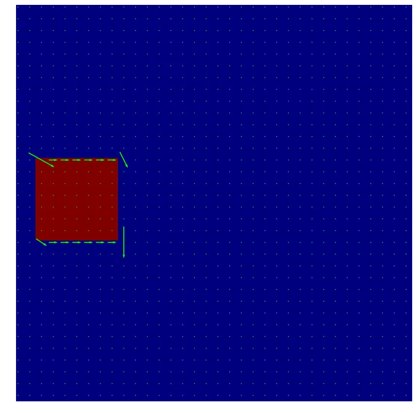
Optical flow on the synthetic box pair. Arrows point down and to the right, matching the 1-pixel shift. Subsampled every 3 pixels.
The arrows at the edges of the box point down-right, which is the correct direction. The interior of the box has no arrows because there’s no gradient there (it’s all white). Same for the black background. Flow is only computable where there’s an intensity edge.