Tracking Objects with Covariance and Mean-Shift
Covariance-based object matching with generalized eigenvalues, and mean-shift tracking with Epanechnikov-weighted color histograms.
Abstract#
Two object tracking methods implemented from scratch. The first matches a given covariance matrix against every patch in an image using generalized eigenvalues as a distance metric. The second tracks a red car across two frames using mean-shift with Epanechnikov-weighted color histograms. The covariance tracker is a brute-force scan. The mean-shift tracker iterates toward the best histogram match, though after 25 iterations it starts drifting off the target.
Covariance tracking#
The idea: you have a model covariance matrix (given in the assignment) that describes some unknown target. You slide a window across the image, compute the covariance matrix of each patch, and find the patch whose covariance is closest to the model. The feature vector per pixel is , so the covariance matrix is 5x5.
The model matrix was given:
modelCovMatrix = np.array([
    [47.917, 0, -146.636, -141.572, -123.269],
    [0, 408.250, 68.487, 69.828, 53.479],
    [-146.636, 68.487, 2654.285, 2621.672, 2440.381],
    [-141.572, 69.828, 2621.672, 2597.818, 2435.368],
[-123.269, 53.479, 2440.381, 2435.368, 2404.923]])To compute the covariance of a patch, I build the feature vector as a 5-by-N array (where N is the number of pixels in the patch) and pass it to np.cov:
def calc_cov(patch):
    feature_vec = np.zeros((5, patch.shape[0] * patch.shape[1]))
    for i in range(0, patch.shape[0]):
        for j in range(0, patch.shape[1]):
            feature_vec[:, (i * patch.shape[1] + j)] = np.array(
                [i, j, patch[i, j, 0], patch[i, j, 1], patch[i, j, 2]])
return np.cov(feature_vec, bias=True)I pre-allocate feature_vec instead of appending to a list and converting. List append followed by np.array() creates a new list object every iteration, so pre-allocating is faster.
Distance metric#
The distance between two covariance matrices uses generalized eigenvalues. You solve , then the distance is:
def cal_distance(cov_model, cov_candidate):
    ew, ev = sp.linalg.eig(cov_model, cov_candidate)
return np.sqrt((np.log(ew)**2).sum())scipy.linalg.eig with two arguments solves the generalized eigenvalue problem. The log makes the metric symmetric: swapping the two matrices negates the logs, but the squares cancel that out.
Sliding window search#
The scan function slides a window across the image with a stride of patch_size - 4 (so there’s a 4-pixel overlap between adjacent patches):
def scan_patches(image, patch_size):
    result = []
    indices = []
    for i in range(0, image.shape[0], patch_size[0] - 4):
        for j in range(0, image.shape[1], patch_size[1] - 4):
            result.append(image[i:i+patch_size[0], j:j+patch_size[1]])
            indices.append((i, j))
return result, indicesThen loop over all patches, track the minimum distance:
patches, indices = scan_patches(cov_target, (70, 24))

minPos = (0, 0)
minDist = float("inf")

for i in range(len(patches)):
    dist = cal_distance(modelCovMatrix, calc_cov(patches[i]))
    if dist < minDist:
        minPos = indices[i]
        minDist = dist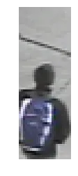
The patch with minimum covariance distance. A boy with a blue bag.
The matched patch is a boy with a blue bag. Or at least that’s what I got, assuming everything was implemented correctly.
Mean-shift tracking#
Mean-shift tracking is a different approach. Build a color histogram of the target region in one frame. In the next frame, start at the same location and iteratively shift the search window toward the position where the color histogram best matches the model. The shift at each step is a weighted mean of pixel positions.
Neighborhood extraction#
Extract all pixels in a region around a center point. The function is called circularNeighbors but it actually extracts a square region (from -radius to radius in both directions). I named it that because the assignment said “circular neighborhood.” The actual circular part comes later in the kernel weighting.
def circularNeighbors(img, x, y, radius):
    F = np.zeros((2*radius*2*radius, 5))
    l = 0
    for i in range(-radius, radius):
        for j in range(-radius, radius):
            F[l] = np.array([(x+i), (y+j),
                img[x+i, y+j, 0], img[x+i, y+j, 1], img[x+i, y+j, 2]])
            l += 1
return FThis returns an Nx5 array where each row is . No bounds checking. The image I was using had the target far enough from the edges that it didn’t matter. In a real system you’d want to handle that, but for a homework, I took the easy route.
Epanechnikov-weighted color histogram#
The color histogram bins the R, G, B channels into a 3D histogram (16 bins per channel, so 16x16x16). Each pixel’s contribution is weighted by the Epanechnikov kernel. Pixels near the center get more weight:
If the value goes negative (pixel is outside the kernel radius), it’s clamped to 0. The histogram is normalized by its sum at the end.
def colorHistogram(X, bins, x, y, h):
    hist = np.zeros((bins, bins, bins))
    for row in X:
        t = 1 - (np.sqrt((row[0]-x)**2 + (row[1]-y)**2) / h)
        t = t**2
        if t < 0:
            t = 0
        hist[int(row[2]//bins), int(row[3]//bins), int(row[4]//bins)] += t
    hist = hist / np.sum(hist)
return histThe bin index for each channel is int(channel_value // bins). With 16 bins and pixel values in [0, 255], this puts values 0-15 in bin 0, 16-31 in bin 1, and so on.
Weight computation#
For each bin , the weight is the square root of the model-to-candidate ratio. If , the weight is 0 (to avoid dividing by zero). Q is the model histogram from the source frame, P is the candidate histogram at the current position in the target frame.
def meanShiftWeights(q_model, p_test, bins):
    w = np.zeros((bins, bins, bins))
    for i in range(bins):
        for j in range(bins):
            for k in range(bins):
                if p_test[i,j,k] == 0:
                    w[i,j,k] = 0
                else:
                    w[i,j,k] = np.sqrt(q_model[i,j,k] / p_test[i,j,k])
return wYes, triple nested loop over 16x16x16 = 4096 bins. Could vectorize it with np.where, but 4096 iterations is nothing.
Tracking loop#
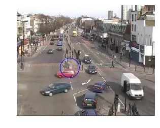
Build the model Q from the source frame (img1.jpg) centered at (150, 175) with radius 25. That’s a red car.
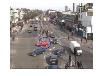
Source frame. Blue circle marks the target: a red car at (150, 175).
Run one iteration first to check the code works:
source = imread('./data/img1.jpg')
cNeigh = circularNeighbors(source, 150, 175, 25)
q_model = colorHistogram(cNeigh, 16, 150, 175, 25)

target = imread('./data/img2.jpg')
tNeigh = circularNeighbors(target, 150, 175, 25)
p_test = colorHistogram(tNeigh, 16, 150, 175, 25)

w = meanShiftWeights(q_model, p_test, 16)The new position after one iteration comes from a weighted sum over the neighborhood. For each offset in [-25, 25), accumulate and , divide by 50, then divide the total by the sum of weights:
out_x = np.zeros((w.shape))
out_y = np.zeros((w.shape))

for i in range(-25, 25):
    out_x += (x_start + i) * w
    out_y += (y_start + i) * w

out_x = out_x / 50
out_y = out_y / 50

new_x = np.sum(out_x) / np.sum(w)
new_y = np.sum(out_y) / np.sum(w)After one iteration: (149.5, 174.5). Barely moved.
Target frame after 1 iteration. Position: (149.5, 174.5).
Then repeat for 25 iterations, updating the center each time:
x_0 = 150.
y_0 = 175.

for iter in range(25):
    tNeigh = circularNeighbors(target, int(x_0), int(y_0), 25)
    p_test = colorHistogram(tNeigh, 16, int(x_0), int(y_0), 25)
    w = meanShiftWeights(q_model, p_test, 16)
    out_x = np.zeros((w.shape))
    out_y = np.zeros((w.shape))
    for i in range(-25, 25):
        out_x += (x_0 + i) * w
        out_y += (y_0 + i) * w
    out_x = out_x / 50
    out_y = out_y / 50
    x_0 = np.sum(out_x) / np.sum(w)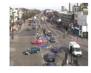
y_0 = np.sum(out_y) / np.sum(w)Final position after 25 iterations: (137.5, 162.5).
After 25 iterations. Final position: (137.5, 162.5).
The tracking followed the car, but the center drifted outside the car’s bounding box. After enough iterations the window starts picking up background pixels and the center gets pulled away. Stopping earlier (maybe 10-15 iterations, or a convergence threshold on the position delta) would probably give a better result.