
Harris Corners, FAST Corners, and OpenCV
Harris corner detector from scratch on a checkerboard, FAST feature detection with a Bresenham circle, and comparing both to skimage.
Abstract#
Two corner detection algorithms implemented from scratch. Harris computes a cornerness score from the structure tensor at every pixel; I tested it on a checkerboard image. FAST checks 16 points on a Bresenham circle around each pixel and looks for contiguous arcs of brighter or darker intensities. Both are compared against skimage’s library implementations at the end, along with Shi-Tomasi.
Harris corner detector#
The Harris detector builds a 2x2 structure tensor at every pixel from the image gradients, then computes a “cornerness” score from it. You compute gradients and with a Gaussian derivative, form the products , , , smooth them with a larger Gaussian, and get from the smoothed products.
Two sigma parameters: for the derivative filter and for the Gaussian window over the products.
Gradients#
gaussian_filter1d from scipy with order=1 gives you a Gaussian derivative in one shot. axis=0 for the x-gradient, axis=1 for y:
sigma_I = 1
sigma_D = 0.7

Ix = gaussian_filter1d(checker, sigma=sigma_D, axis=0, order=1,
                       mode='reflect', cval=0.0, truncate=4.0)
Iy = gaussian_filter1d(checker, sigma=sigma_D, axis=1, order=1,
mode='reflect', cval=0.0, truncate=4.0)Then the products and their Gaussian-smoothed versions:
Ix2 = Ix**2
Iy2 = Iy**2
IxIy = Ix * Iy

gIx2 = gaussian(Ix2, sigma=sigma_I)
gIy2 = gaussian(Iy2, sigma=sigma_I)
gIxIy = gaussian(IxIy, sigma=sigma_I)The Gaussian smoothing here is skimage.filters.gaussian, not the scipy one. These smoothed products are the entries of the structure tensor at each pixel:
Computing R#
The Harris response is:
which expands to:
Wait. Looking at my code again, I actually had a + in front of the term:
R = gIx2*gIy2 - gIxIy**2 + 0.05*(gIx2 + gIy2)**2So I was computing with . The standard formulation subtracts the trace term. I think this still works as a corner measure because both and are large at corners, so adding them just makes the response bigger there. Edges still get suppressed because the determinant is near zero for edges regardless.
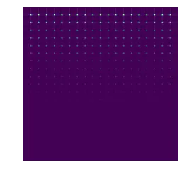
Harris R response. Bright spots are candidate corners.
The R values are large. Printing R[17:23, 17:23] gives values up to ~76 million. So the threshold needs to be correspondingly large.
Thresholding#
Subtract 1,000,000 and clamp negatives to zero:
R_fix = R - 1000000
R_fix[R_fix < 0] = 0
R after thresholding at 1,000,000.
Non-maximal suppression#
I tried doing this as a convolution with generic_filter from scipy first, passing a function that returns the center pixel only if it’s the max. That was wrong, so I scrapped it.
The actual version loops over every interior pixel and checks whether it’s the unique maximum in its 3x3 neighborhood:
def checkIfUniqueMax(image, row, col):
    m = np.max(image[row-1:row+2, col-1:col+2])
    c = 0
    for i in range(row-1, row+2):
        for j in range(col-1, col+2):
            if image[i][j] == m:
                c += 1
    return image[row][col] == m and c == 1

def nonmaxSuppress(image):
    corners = []
    rows, cols = image.shape
    for row in range(1, rows-1):
        for col in range(1, cols-1):
            if checkIfUniqueMax(image, row, col):
                corners.append((col, row))
return corners“Unique max” means the center pixel is strictly greater than all 8 neighbors. If two adjacent pixels have the same value, neither gets kept. The corners come back as (col, row) tuples for plotting with scatter.

Corners after non-maximal suppression on the thresholded R.
The NMS actually revealed some corners that were hidden in the thresholded R image. My hypothesis: the non-maximal suppression is playing around with the eigenvalue regions from the slides, making the decision boundary look more like Shi-Tomasi’s boxed layout rather than the conical layout of Harris. That would explain why the library Shi-Tomasi detector (below) gives comparable results to my Harris + NMS.
FAST feature detector#
FAST checks 16 points on a Bresenham circle of radius 3 around each candidate pixel. If or more contiguous points on that circle are all brighter (or all darker) than the center by some threshold, it’s a corner.
The circle#
I hardcoded the 16 offsets. Point 16 is the same as point 1 (both are (row+3, col)), so the function actually returns 15 points:
def circle(row, col):
    point1  = (row+3, col)
    point2  = (row+3, col+1)
    point3  = (row+2, col+2)
    point4  = (row+1, col+3)
    point5  = (row,   col+3)
    point6  = (row-1, col+3)
    point7  = (row-2, col+2)
    point8  = (row-3, col+1)
    point9  = (row-3, col)
    point10 = (row-3, col-1)
    point11 = (row-2, col-2)
    point12 = (row-1, col-3)
    point13 = (row,   col-3)
    point14 = (row+1, col-3)
    point15 = (row+2, col-2)
    return [point1, point2, point3, point4, point5, point6, point7,
            point8, point9, point10, point11, point12, point13,
point14, point15]Not elegant, but it’s a lookup table. The whole point of FAST is that these offsets are fixed.
Corner test#
Each circle point gets classified: 1 if brighter than center + threshold, 2 if darker than center - threshold, 0 otherwise. Then I need to find the longest contiguous run of the same non-zero label.
The wraparound problem: the circle is circular but the array is linear. If points 14, 15, 1, 2 are all “brighter,” that run of 4 spans the array boundary. I handled it by doubling the classification array (appending it to itself) and doing a single linear scan:
def is_corner(image, row, col, ROI, threshold, n_star):
    intensity = int(image[row][col])
    circ = []
    for el in ROI:
        if image[el[0]][el[1]] > intensity + threshold:
            circ.append(1)
        elif image[el[0]][el[1]] < intensity - threshold:
            circ.append(2)
        else:
            circ.append(0)
    # duplicate to handle wraparound
    for el in ROI:
        if image[el[0]][el[1]] > intensity + threshold:
            circ.append(1)
        elif image[el[0]][el[1]] < intensity - threshold:
            circ.append(2)
        else:
            circ.append(0)

    el = circ[0]
    count = 1
    largest_ct = count
    for i in range(1, len(circ)):
        if circ[i] == el and circ[i] != 0:
            count += 1
        else:
            if circ[i] != 0:
                if largest_ct < count:
                    largest_ct = count
                count = 1
                el = circ[i]
            if circ[i] == 0:
                el = 0

return largest_ct >= n_starIf a run wraps around the boundary, it shows up as a long run in the middle of the doubled array. No modular arithmetic needed.
Detection loop#
Search every pixel with a 3-pixel border (since the circle has radius 3), using :
def detect(image, threshold=50):
    corners = []
    rows, cols = image.shape
    for row in range(3, rows-3):
        for col in range(3, cols-3):
            ROI = circle(row, col)
            if is_corner(image, row, col, ROI, threshold, n_star=9):
                corners.append((col, row))
return cornersTested with thresholds 10, 20, 30, 50:
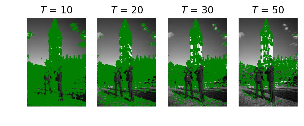
FAST corner detection at T = 10, 20, 30, 50.
At T=10 almost everything lights up. At T=50 only the strongest edges survive. Results look similar to the slides and to the library version below. The library version only checks a subset of the 16 points (a speed-test lookup table), so it’s way faster, but on this image the output is about the same.
Library comparisons#
skimage Harris#
from skimage.feature import corner_harris, corner_peaks, corner_subpix
coords = corner_peaks(corner_harris(checker), min_distance=1)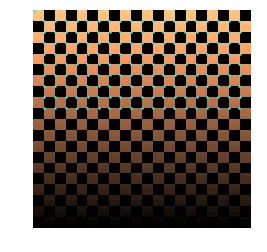
skimage corner_harris + corner_peaks on the checkerboard.
They get results similar to what I had before NMS. They miss some of the lower corners because their peak detection is different from my “unique max” approach.
skimage Shi-Tomasi#
from skimage.feature import corner_shi_tomasi
coords = corner_peaks(corner_shi_tomasi(checker), min_distance=1)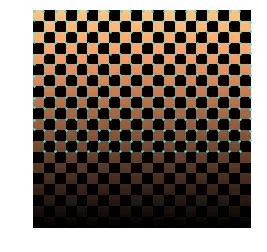
skimage corner_shi_tomasi on the checkerboard.
Shi-Tomasi gives results comparable to my Harris + NMS. Supports the idea that NMS is pushing the Harris boundary toward Shi-Tomasi territory.
skimage FAST#
from skimage.feature import corner_fast
coords = corner_peaks(corner_fast(tower, 10), min_distance=1)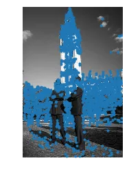
skimage corner_fast on the tower, threshold=10.
Similar results at the same threshold, but way faster. Argument could be made about it tripping up on a more complex image, but on this tower the difference is negligible.