
Backpropagation and the N-Bit Parity Problem
Implementing a multi-layer perceptron from scratch to solve the N-bit parity problem, and analyzing the effects of learning rate and momentum.
First project for CSE 5526: Introduction to Neural Networks (Autumn 2018). After the homeworks covered M-P neurons and the perceptron learning rule, this project had us implement a full multi-layer perceptron (MLP) from scratch and train it with backpropagation.
The N-Bit Parity Problem#
The N-bit parity function outputs 1 if the number of 1-bits in the input is odd, and 0 otherwise. For example, with :
- (two 1-bits) 0 (even parity)
- (three 1-bits) 1 (odd parity)
What makes this hard for a neural network is that every input bit matters, and flipping any single bit changes the output. There’s no local structure to exploit. The network has to learn a truly global function over all inputs, which is why parity is a standard benchmark for training algorithms.
For , the training set is all binary numbers (0 through 15).
Network Architecture#
The MLP uses a two-layer feedforward architecture with sigmoid activation:
Layer 1 (hidden): Takes the -bit input (plus a bias term) and produces hidden units.
- Weight matrix:
Layer 2 (output): Takes the hidden layer output (plus a bias term) and produces a single output.
- Weight matrix:
Forward propagation:
where is the sigmoid activation function, and denotes prepending a bias term.
Backward propagation computes the error gradients using the sigmoid derivative , which simplifies nicely when expressed in terms of the output: .
For the output layer:
For the hidden layer:
Weight updates incorporate optional momentum ():
Convergence criterion: All 16 outputs must be within 0.05 of their desired values.
Implementation#
The implementation is a self-contained MultiLayerPerceptron class in Python/NumPy:
import numpy as np

def sigmoid(z):
    return 1 / (1 + np.exp(-z))

class MultiLayerPerceptron:
    def __init__(self, parity=4, eta=0.2, alpha=0):
        self.parity = parity
        self.eta = eta
        self.alpha = alpha
        self.W = [
            np.random.uniform(-1, 1, (parity+1, parity)),
            np.random.uniform(-1, 1, (parity+1, 1))
        ]
        self.delta_W = [np.zeros_like(w) for w in self.W]
        self.X, self.D = self._get_train_data()

    def forwardProp(self, x):
        h = sigmoid(np.dot(self.W[0].T, x))
        y = sigmoid(np.dot(self.W[1].T, np.insert(h, 0, 1, axis=0)))
        return [h, y]

    def backwardProp(self, x, Y, d_k):
        y_k = Y[1]
        delta_k = y_k * (1 - y_k) * (d_k - y_k)

        self.delta_W[1] = (self.eta * delta_k.T
                           * np.insert(Y[0], 0, 1, axis=0)
                           + self.alpha * self.delta_W[1])
        delta_j = Y[0] * (1 - Y[0]) * self.W[1][1:] * delta_k

        self.delta_W[0] = (self.eta * delta_j.T * x
                           + self.alpha * self.delta_W[0])
        self.W[0] += self.delta_W[0]
self.W[1] += self.delta_W[1]I also parallelized the training using Python’s multiprocessing module, since each configuration (learning rate + momentum combination) is independent and can run on its own core.
Experimental Results#
I swept learning rates from 0.05 to 0.50 (in steps of 0.05), both without momentum () and with momentum ().
Without Momentum ()#
| Epochs | |
|---|---|
| 0.05 | 35,869 |
| 0.10 | 16,477 |
| 0.15 | 12,681 |
| 0.20 | 9,541 |
| 0.25 | 8,719 |
| 0.30 | 6,180 |
| 0.35 | 5,319 |
| 0.40 | 5,121 |
| 0.45 | 6,683 |
| 0.50 | 120,389 |
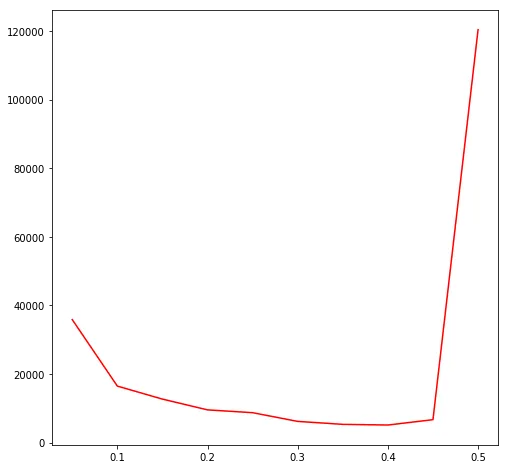
There’s a clear sweet spot. Increasing from 0.05 to 0.40 steadily reduces the number of epochs needed. But past 0.40, the step size gets too large and the network overcompensates for each error, causing weight oscillations that slow convergence way down. At , it takes over 120,000 epochs, which is a 23x regression from the optimal.
With Momentum ()#
| Epochs | |
|---|---|
| 0.05 | 3,206 |
| 0.10 | 1,791 |
| 0.15 | 1,139 |
| 0.20 | 975 |
| 0.25 | 878 |
| 0.30 | 623 |
| 0.35 | 547 |
| 0.40 | 514 |
| 0.45 | 5,197 |
| 0.50 | 9,878 |
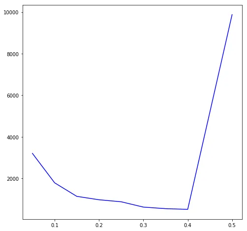
Momentum gives a consistent and big speedup without changing the overall shape of the curve. The optimal is still 0.40, but the network converges in 514 epochs instead of 5,121.
Momentum Speedup Analysis#
| Without | With | Speedup | |
|---|---|---|---|
| 0.05 | 35,869 | 3,206 | 11.2x |
| 0.10 | 16,477 | 1,791 | 9.2x |
| 0.15 | 12,681 | 1,139 | 11.1x |
| 0.20 | 9,541 | 975 | 9.8x |
| 0.25 | 8,719 | 878 | 9.9x |
| 0.30 | 6,180 | 623 | 9.9x |
| 0.35 | 5,319 | 547 | 9.7x |
| 0.40 | 5,121 | 514 | 10.0x |
| 0.45 | 6,683 | 5,197 | 1.3x |
| 0.50 | 120,389 | 9,878 | 12.2x |
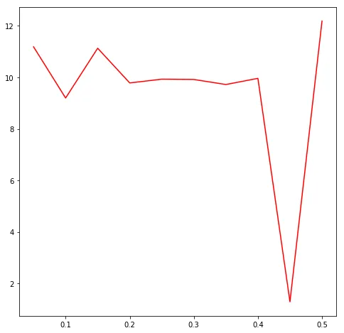
The speedup is pretty consistent at around 10x across most learning rates. The weird outlier is , where momentum only gives a 1.3x speedup. My guess is that this is a transitional zone: the learning rate is just large enough to cause instability on its own, and momentum (which increases the effective step size) tips it over into oscillatory behavior. What’s interesting is that at the even higher , momentum gets its 12x speedup back, which suggests a different dynamical regime.
What I Took Away#
Learning rate turned out to be the most important hyperparameter by far. The difference between a good and bad choice was orders of magnitude in convergence time, and the transition from “working fine” to “taking forever” was pretty abrupt (0.40 to 0.50).
Momentum gave a solid ~10x speedup most of the time, but it’s not a free parameter to crank up. The case showed that momentum and learning rate can interact badly: the combined effective step size is what actually matters, not either parameter in isolation.
The parity problem itself was a good choice for this project. Because every input bit affects the output, every neuron has to participate in every decision. You can’t get away with some neurons being “lazy.” I also appreciated having to implement backpropagation by hand, computing for the output layer, propagating back through the hidden layer, wiring in momentum. It’s not hard to use a framework for this stuff, but doing it manually once made the algorithm feel a lot more concrete.