Perceptron Learning, the XOR Problem, and Gradient Descent

Second homework for CSE 5526: Introduction to Neural Networks (Autumn 2018). The first homework was about what M-P neurons can represent; this one was about how they learn, and where learning breaks.

Problem 1: The Perceptron Learning Rule#

Part (a): Linear Classification#

Four training samples in $\{0, 1\}$ space:

$x_1 = (0,0)^T \in C_1, \quad x_2 = (0,1)^T \in C_1, \quad x_3 = (1,0)^T \in C_2, \quad x_4 = (1,1)^T \in C_2$

We had to apply the perceptron learning rule with $\eta = 0.5$ and $w(0) = (0, 0, 0)^T$ (third component is the bias weight).

I converted the points from $[0,1]$ to $\{-1,1\}$ space using $g(x) = 2x - 1$ to keep things consistent with the M-P neuron model from the last homework. The learning rule is:

$w(n+1) = w(n) + \eta(d - w(n)^T x) \cdot x$

First epoch:

$w(1) = (0,0,0)^T + 0.5(-1-1)(-1,-1,1)^T = (1,1,-1)^T$ $w(2) = (1,1,-1)^T + 0.5(-1+1)(-1,1,1)^T = (1,1,-1)^T$ $w(3) = (1,1,-1)^T + 0.5(1+1)(1,-1,1)^T = (2,0,0)^T$ $w(4) = (2,0,0)^T + 0.5(1-1)(1,1,1)^T = (2,0,0)^T$

Second epoch: no weights change, so we stop. The decision boundary ends up being $x_1 = 0$ (or $x_1 = 0.5$ in the original space), which is just a vertical line separating the classes. It converges in 2 epochs.

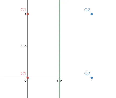
Part (b): The XOR Problem#

Same four points, but now $x_2, x_3 \in C_1$ and $x_1, x_4 \in C_2$. This is XOR.

Running the perceptron learning rule:

$w(1) = (0,0,0)^T + 0.5(-1-1)(-1,1,1)^T = (1,-1,-1)^T$ $w(2) = (1,-1,-1)^T + 0.5(1+1)(1,1,1)^T = (1,-1,-1)^T$ $w(3) = (1,-1,-1)^T + 0.5(1+1)(-1,-1,1)^T = (0,-2,0)^T$ $w(4) = (0,-2,0)^T + 0.5(-1+1)(-1,1,1)^T = (0,-2,0)^T$

After another epoch, the weights cycle back to $(0,0,0)^T$ and we’re right where we started. It loops forever.

This makes sense: XOR is not linearly separable. No single line can divide the plane so that $(0,0)$ and $(1,1)$ are on one side and $(0,1)$ and $(1,0)$ are on the other. The perceptron convergence theorem only guarantees convergence for linearly separable data, so when the data isn’t separable, the algorithm just oscillates. This is the classic result that Minsky and Papert pointed out, and it’s why multi-layer networks became necessary.

Problem 2: Multi-Layer Perceptron for Non-Linearly Separable Classes#

This problem had four classes in 2D that can’t be separated by single linear boundaries. We had to design a two-layer feedforward M-P network with three output units.

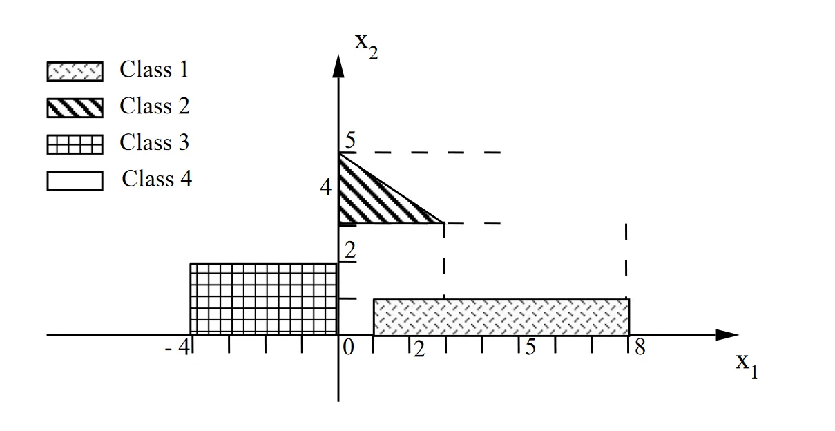
My approach was to decompose each class into a region defined by linear inequalities:

Class 1: $(x_1 \geq 1) \land (x_1 \leq 8) \land (x_2 \geq 0) \land (x_2 \leq 1)$

Class 2: $(x_1 \geq -4) \land (x_1 \leq 0) \land (x_2 \geq 0) \land (x_2 \leq 2)$

Class 3: $(x_1 \geq 0) \land (x_1 \leq 3) \land (x_2 \geq 3) \land (x_2 \leq 5) \land (15 - 2x_1 - 3x_2 \geq 0)$

Class 4: Everything else (all $y_i = -1$).

Each inequality is handled by one neuron in the first layer. The second layer takes these outputs and ANDs them together for each class. So the first layer does half-plane decisions and the second layer combines them into the polygonal/rectangular regions.

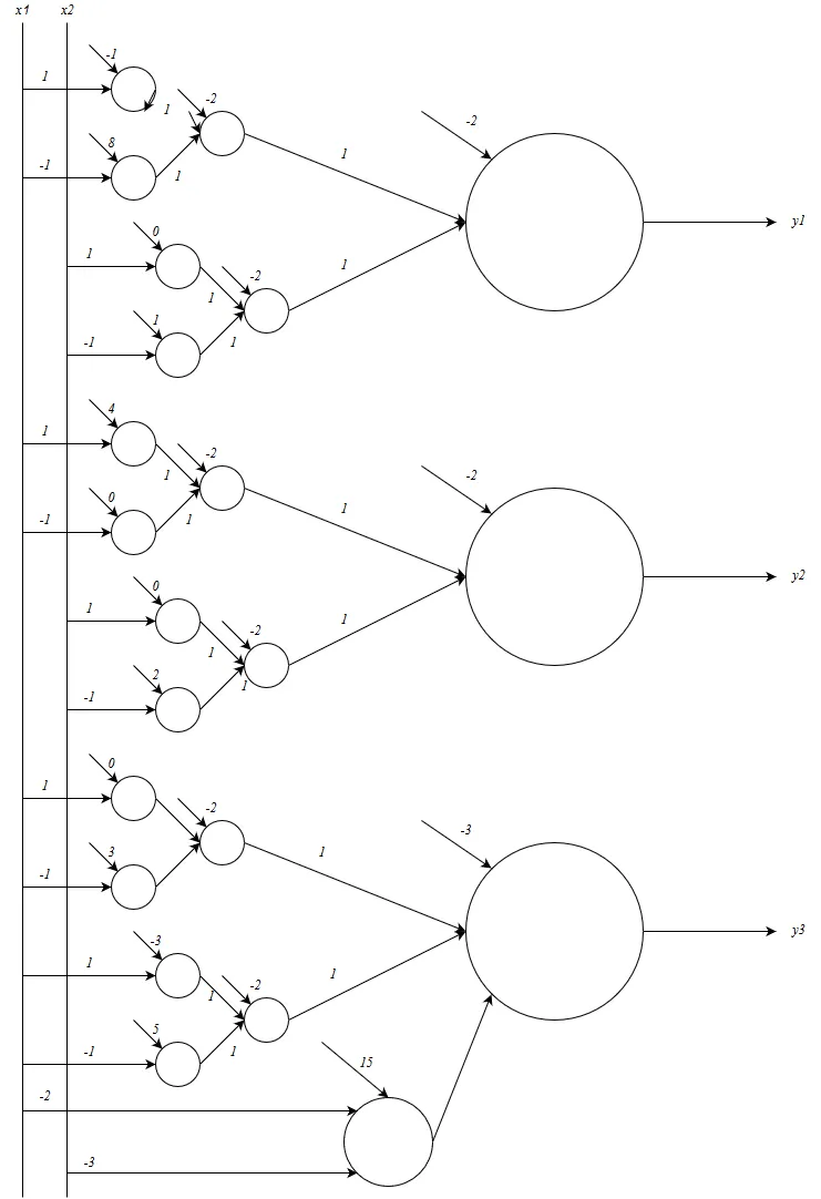
This is basically what the XOR problem was hinting at: you need multiple layers to carve out non-convex or non-linearly-separable regions. The first layer creates the individual boundaries and the second layer composes them.

Problem 3: Cost Functions, Gradients, and LMS#

Given input-output pairs:

$X = \{-0.5, -0.2, -0.1, 0.3, 0.4, 0.5, 0.7\}$ $D = \{-1, 1, 2, 3.2, 3.5, 5, 6\}$

We needed to write down the cost function with respect to $w$ (bias = 0), then compute the gradient at $w = 2$ using direct differentiation and LMS approximation, and see if they agree.

Cost function:

$E = \frac{1}{2} \sum (D - wX)^2$

Direct differentiation:

$\nabla E = \sum X(-D + wX)$

At $w = 2$: $\nabla E\big|_{w=2} = \sum X(-D + 2X)$

LMS approximation:

$\nabla E(n) = -e(n) \cdot x(n) \quad \text{where } e(n) = d(n) - w \cdot x(n)$

Both give a mean gradient of -0.94 and a sum of -6.58.

import numpy as np
x = np.array([-0.5, -0.2, -0.1, 0.3, 0.4, 0.5, 0.7])
d = np.array([-1, 1, 2, 3.2, 3.5, 5, 6])
w = 2
gradient = -np.mean(np.multiply(np.subtract(d, w*x), x))
directdiff = np.mean(np.multiply(x, -d + 2*x))
print(f"LMS gradient = {gradient}")      # -0.94
print(f"Direct diff  = {directdiff}")     # -0.94

They agree because the data is linear and the model is linear, so the exact differential and the LMS approximation are computing the same thing. For non-linear data or a model that can’t fully express the relationship, LMS would start to deviate.

What I Took Away#

The XOR result was probably the most memorable part of this homework. It’s one thing to read that single-layer perceptrons can’t learn XOR, but actually watching the weights cycle back to zero and loop forever makes it concrete. The multi-layer network design in problem 2 then showed how adding a layer fixes the issue: first layer draws the lines, second layer combines them.

The gradient/LMS comparison in problem 3 was also useful for building intuition. I hadn’t thought much about when the LMS approximation is exact vs. approximate before this, and it turns out the answer is straightforward: they match when the model is expressive enough for the data.