Linear Regression and Bayes Decision Boundaries • TheAnig

Abstract#

Three problems from the first ML homework. Fit a line with ordinary least squares, compute the probability of error for a Bayesian classifier using the error function, and plot the Bayes decision boundary for two multivariate Gaussians. All synthetic data, all NumPy.

This was the first homework for a graduate machine learning course. The problems were meant to get us comfortable with the math before anything got complicated. Everything here is closed-form or direct computation. No optimization loops, no hyperparameters.

Ordinary least squares regression#

The setup: generate 1000 training samples from the model $y = 1 - 0.5x + z$ where $x \sim \mathcal{N}(0, 1)$ and $z \sim \mathcal{N}(0, 0.01)$ . Then fit a linear model using the normal equation and see how close the estimated weights land to the true ones.

The design matrix $X$ has a column of ones prepended for the intercept:

x = np.random.randn(1000, 1)
ones = np.ones((1000, 1))
X = np.append(ones, x, axis=1)
z = sqrt(0.01) * np.random.randn(1000, 1)

y = 1 - (0.5 * x) + z

python

The OLS solution is the closed-form weight vector:

$w = (X^T X)^{-1} X^T y$

w = np.linalg.inv(X.T.dot(X)).dot(X.T.dot(y))

python

The estimated weights came out to $w = [1.00264, -0.49771]$ , which is close to the true $[1, -0.5]$ . With 1000 samples and low noise variance (0.01), there isn’t much room for the estimate to drift.

Training MSE was 0.0106 and test MSE (on 100 fresh samples) was 0.0091. The test error being lower than training error might look odd, but with only 100 test points it’s just sampling noise. Both are close to the noise variance of 0.01, which is the irreducible error floor for this problem.

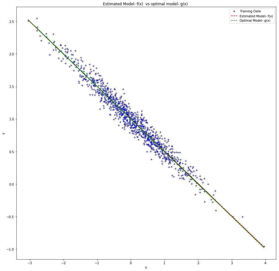
Training data with estimated and optimal regression lines — Blue crosses are training data. The red dashed line is the estimated model $f(x) = 1.003 - 0.498x$ . The green dashed line is the true model $g(x) = 1 - 0.5x$ . They overlap almost completely.

The two lines are nearly indistinguishable. That’s the whole point. With a correctly specified model and enough data relative to the noise, OLS recovers the true parameters.

Bayes error probability#

This problem asked for the probability of error of a Bayesian classifier. Two classes with prior probabilities 0.7 and 0.3, both Gaussian. The decision regions are determined by the likelihood ratio, and the error integral involves the Gaussian CDF, which is where math.erf comes in.

The error function relates to the Gaussian CDF by:

$\Phi(x) = \frac{1}{2}\left[1 + \text{erf}\left(\frac{x}{\sqrt{2}}\right)\right]$

The computation boils down to plugging in the standardized decision boundary thresholds:

import math

pr_error = (0.7 * (1 - (0.5 * (math.erf(0.8302) + math.erf(3.659))))
            + (0.3 / 2.0) * (math.erf(3.5869) - math.erf(0.4130)))

python

Result: $P(\text{error}) \approx 0.168$ . About 16.8% of samples will be misclassified even by the optimal Bayes classifier. This is the best any classifier can do given the overlap between the two class distributions. The asymmetric priors (0.7/0.3) shift the decision boundary toward the less likely class, but there’s still enough overlap in the tails to guarantee some errors.

Bayes decision boundary for two Gaussians#

Last problem: generate 1000 samples from each of two 2D Gaussians and plot the Bayes decision boundary.

Class $y = +1$ : mean $= [1, 0]$ , covariance $= \begin{bmatrix} 1 & -1 \\ -1 & 4 \end{bmatrix}$
Class $y = -1$ : mean $= [-1, 1]$ , covariance $= \begin{bmatrix} 1 & -1 \\ -1 & 4 \end{bmatrix}$

The covariance matrices are the same for both classes. When the covariances are equal, the Bayes boundary is linear. You can derive it by setting the log-posterior ratio to zero:

$\frac{7}{3}x_1 + \frac{1}{3}x_2 + \ln\left(\frac{2}{3}\right) - \frac{1}{6} = 0$

The $\ln(2/3)$ term comes from unequal priors.

mean_pos = [1, 0]
mean_neg = [-1, 1]
cov = [[1, -1], [-1, 4]]

p_x_y1 = np.random.multivariate_normal(mean_pos, cov, 1000)
p_x_y_minus1 = np.random.multivariate_normal(mean_neg, cov, 1000)

x1 = np.linspace(-5, 5, 1000)
x2 = np.linspace(-5, 5, 1000)
line = (7.0/3.0) * x1 + (1.0/3.0) * x2 + math.log(2.0/3.0) - (1.0/6.0)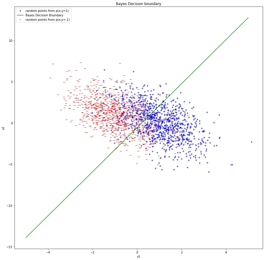

python

Bayes decision boundary with two classes of samples — Blue and red points are the two classes. The green line is the Bayes decision boundary.

There’s considerable overlap between the two classes because of the large variance along $x_2$ (the $(2,2)$ entry of the covariance is 4). The negative covariance of $-1$ tilts the distributions, so the boundary cuts diagonally.

The boundary derivation is an exercise in multivariate Gaussian algebra. With equal covariances, the quadratic terms cancel and you’re left with a linear boundary. If the covariances were different, you’d get a quadratic (parabola, ellipse, or hyperbola depending on the geometry). That case shows up in the next homework.